Aggregate climate data to DHIS2 organisation units

In this notebook we will show how to load daily climate data from NetCDF and use earthkit to aggregate temperature and precipitation climate variables to DHIS2 organisation units.

import geopandas as gpd
import xarray as xr
from earthkit import transforms

Loading the data¶

Our sample NetCDF file contains ERA5-Land monthly temperature and precipitation data for Sierra Leone between 1990 and 2025. Let’s load the file using xarray and drop some variables that we don’t need:

file = "../data/era5-land-monthly-temp-precip-1990-2025-sierra-leone.nc"
data = xr.open_dataset(file)
data = data.drop_vars(['number', 'expver'])

If we inspect the xarray dataset, we see that the file includes 2 spatial dimensions (latitude, longitude), a temporal dimension containing 428 months (valid_time) and two data variables t2m (temperature at 2m above sea level), and tp (total precipitation). The data source is European Centre for Medium-Range Weather Forecasts (ECMWF).

data

Loading the organisation units¶

Next, we use GeoPandas to load our organisation units that we’ve downloaded from DHIS2 as a GeoJSON file:

district_file = "../data/sierra-leone-districts.geojson"
org_units = gpd.read_file(district_file)

The GeoJSON file contains the boundaries of 13 named organisation units in Sierra Leone. For the aggregation, we are particularly interested in the id and the geometry (polygon) of the org unit:

org_units

Aggregating the data to organisation units¶

To aggregate the data to the org unit features we use the spatial.reduce function of earthkit-transforms. We keep the daily period type and only aggregate the data spatially to the org unit features.

Since our climate data variables need to be aggregated using different statistics, we do separate aggregations for each variable.

Temperature¶

First, let’s see what the temperature data looks like that we are trying to aggregate. We select July 2025 and plot it on a map:

data.sel(valid_time='2025-07')['t2m'].plot(cmap='YlOrRd')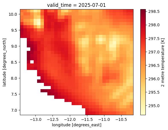

To aggregate the temperature variable, we extract the temperature or t2m variable, and tell the spatial.reduce function to aggregate the data to our organisation units org_units. We set mask_dim='id' to specify that we want one aggregated value for every unique value in the organisation unit id column. Finally, we set how='mean' so that we get the average temperature of all gridded values that land inside an organisation unit.

temp = data['t2m']
agg_temp = transforms.spatial.reduce(temp, org_units, mask_dim='id', how='mean')
agg_temp.sizes

Frozen({'id': 13, 'valid_time': 428})

The result from spatial.reduce is an xarray object and contains data for 13 organisation units along the id dimensions, and 428 months along the valid_time dimension. To more easily read the aggregated values, we convert it to a Pandas DataFrame:

agg_temp_df = agg_temp.to_dataframe().reset_index()
agg_temp_df

We see that the aggregated dataframe contains what seems to be kelvin temperature values for each organisation unit and each time period (monthly).

Finally, let’s plot what this looks like on a map. We can merge our Pandas DataFrame with the org_units GeoPandas DataFrame to plot the aggregated temperature values on a map. We again select July 2025 to compare with the previous map of gridded temperature values for the same date.

agg_temp_snapshot = agg_temp_df[agg_temp_df['valid_time']=='2025-07']
org_units_with_temp = org_units.merge(agg_temp_snapshot, on='id', how='left')
org_units_with_temp.plot(column="t2m", cmap="YlOrRd", legend=True)

<Axes: >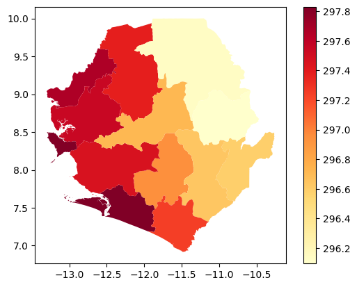

Precipitation¶

Important: The monthly version of ERA5-Land reports all variables as daily averages. In order to get total precipitation for the entire month, we should first multiply the average daily precipitation (tp) with the number of days per month (xarray date fields provide this as an attribute .dt.days_in_month):

data['tp'] = data['tp'] * data.valid_time.dt.days_in_month

Let’s see what the total precipitation data for July 2025 looks like on a map:

data.sel(valid_time='2025-07')['tp'].plot(cmap='YlGnBu')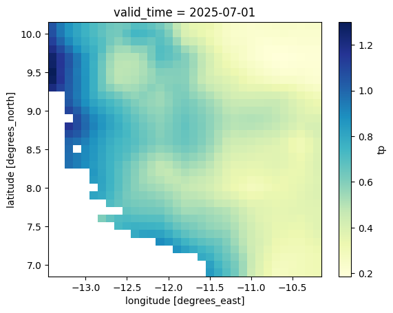

We then use the same aggregation approach by selecting and passing the tp variable to the transforms.spatial.reduce function. We set how='mean' to get the average precipitation for the entire area. It’s also common to report minimum and maximum precipitation, which can be done by instead setting how='min' or how='max'.

precip = data['tp']
agg_precip = transforms.spatial.reduce(precip, org_units, mask_dim='id', how='mean')
agg_precip_df = agg_precip.to_dataframe().reset_index()
agg_precip_df

We see that the aggregated dataframe contains what seems to be total precipitation values in meters for each organisation unit and each time period (monthly).

Again, we can convert our xarray to a merged GeoPandas DataFrame to map aggregated precipitation values for July 2025:

agg_precip_snapshot = agg_precip_df[agg_precip_df['valid_time']=='2025-07']
org_units_with_precip = org_units.merge(agg_precip_snapshot, on='id', how='left')
org_units_with_precip.plot(column="tp", cmap="YlGnBu", legend=True)

<Axes: >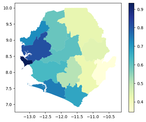

Post-processing¶

We have now aggregated the temperature and precipitation data to our organisation units. But before we submit the results to DHIS2, we want to make sure they are reported in a format that makes sense to most users.

For temperature, we convert the data values from kelvin to Celcius by subtracting 273.15 from the values:

agg_temp_df['t2m'] -= 273.15
agg_temp_df

For precipitation, to avoid small decimal numbers, we convert the reporting unit from meters to millimeters:

agg_precip_df['tp'] *= 1000
agg_precip_df

Next steps¶

In this notebook, we have successfully aggregated temperature and precipitation data into Pandas DataFrames and converted the values to more easily interpreted units such as degrees Celsius and millimeters. To learn how to import these aggregated DataFrames into DHIS2, see our guide for importing data values using the Python DHIS2 client.